
Of Spectrograms and Discriminators
Everything I learned so far about audio models and tokenization

Most of my fellow youngins in artificial intelligence talk about the latest trendy stuff: agents, diffusion, reinforcement learning, et al. But since audio is my thing and I’m sticking with it for several reasons, I chose to spend my limited time and only compute (1xMI300X, courtesy Hot Aisle) tinkering with audio projects.
Introduction
First, I want to start by highlighting the most important difficulty in modeling audio with a neural network, which is the massive length: just one second of 16KHz audio alone is already… sixteen thousand samples — the Greek kilo in kilohertz stands for a thousand. CD quality audio starts at 44.1 kilohertz: therefore, just ten seconds of 44.1KHz audio is already 441 thousand samples.
The most normal “raw” way to represent audio is through PCM (Pulse Code Modulation), which represents each sample as 16-bit signed integers (-32,768 to +32,767). In 99% of cases machine learning-wise, each sample is turned into a float of range [-1.0, 1.0], by dividing by the maximum possible integer value.
All this means, to predict ten seconds of 44.1KHz audio, your model must output a 1D sequence of 441,000 floats. For comparison, if you wanted to output an RGB 256x256 image, you’d need just 256 x 256 x 3 = 196,608 floats.
So, considering all this, how did people cope?
Brief History: WaveNet to GANs
Legacy Approaches
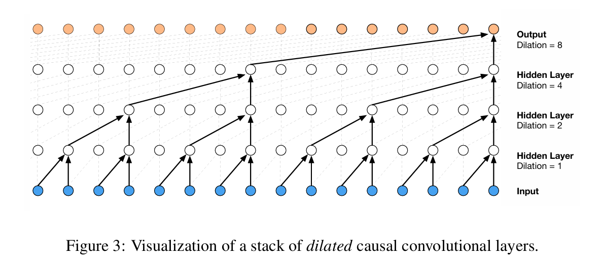
The story of neural audio generation started with WaveNet (DeepMind, 2016). It showed that by stacking dilated causal convolutions, you could generate raw audio directly, sample by sample, with great quality compared to previous approaches. The catch? It was SLOW
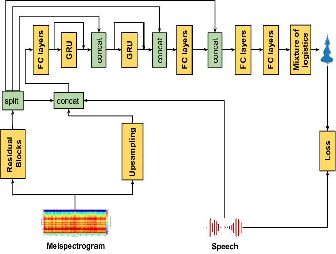
In 2018 came WaveRNN, which used a GRU and clever softmax tricks to achieve 4x realtime, high quality 24KHz audio synthesis, and even real time on a mobile CPU after pruning up to 96% of the weights with minimal quality loss.
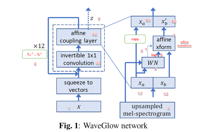
At the same time WaveGlow (NVIDIA) appeared, where it ditched autoregression and proposed a fully parallel approach based on invertible flows.
Now, most people don’t model audio just for the hell of it, but for predicting some orderly sequence, like speech from text — or later, music from text. For that, having the expensive structured model directly predict audio was impractical, so people settled for some sort of intermediate representation. At this point of time (2018-2021), it was the mel spectrogram:
The mel spectrogram hit a sweet spot. First, it compresses raw waveforms by orders of magnitude, turning tens of thousands of samples into a 2D time-frequency “image” that’s much easier for neural networks to predict. Second, it coincides with human perception: the mel scale approximates how our ears resolve pitch and frequency, making it perceptually meaningful.
However, the mel spectrogram is a very lossy representation, as it compresses magnitude info and straight up discards phase. Therefore, most of the models I mentioned before (and will later) are used as neural vocoders: take mel spectrogram, reconstruct audio. Here’s an example:
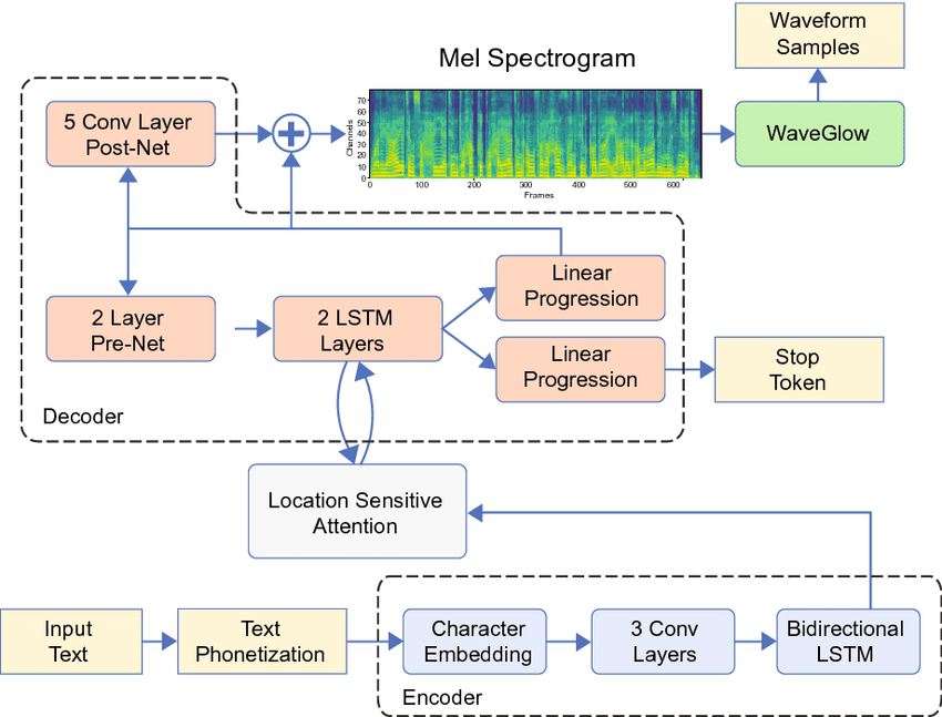
The diagram above is of Tacotron 2 + WaveGlow, which was the dominating stack in text-to-speech for quite a bit. Tacotron 2 was an RNN (LSTM)-based encoder-decoder network that used location sensitive attention to align phonemes or text to mel spectrogram, which would then be fed into the neural vocoder to extract audio.
Rise of the GAN vocoders
WaveGlow, the last non-GAN approach, was fast compared to WaveNet, but something was about to blow it away.
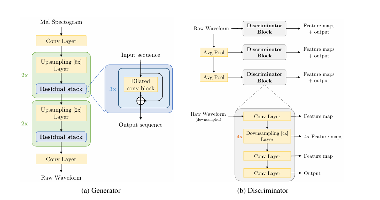
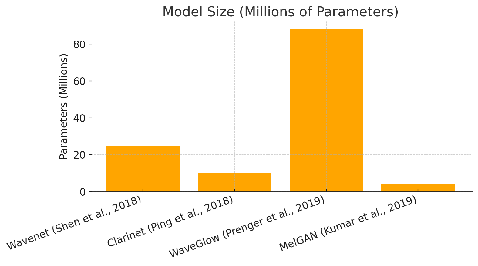
Enter MelGAN (2019), which wasn’t technically the very first audio GAN, but the first one to actually succeed. Most notably, MelGAN was 10x faster than WaveGlow.
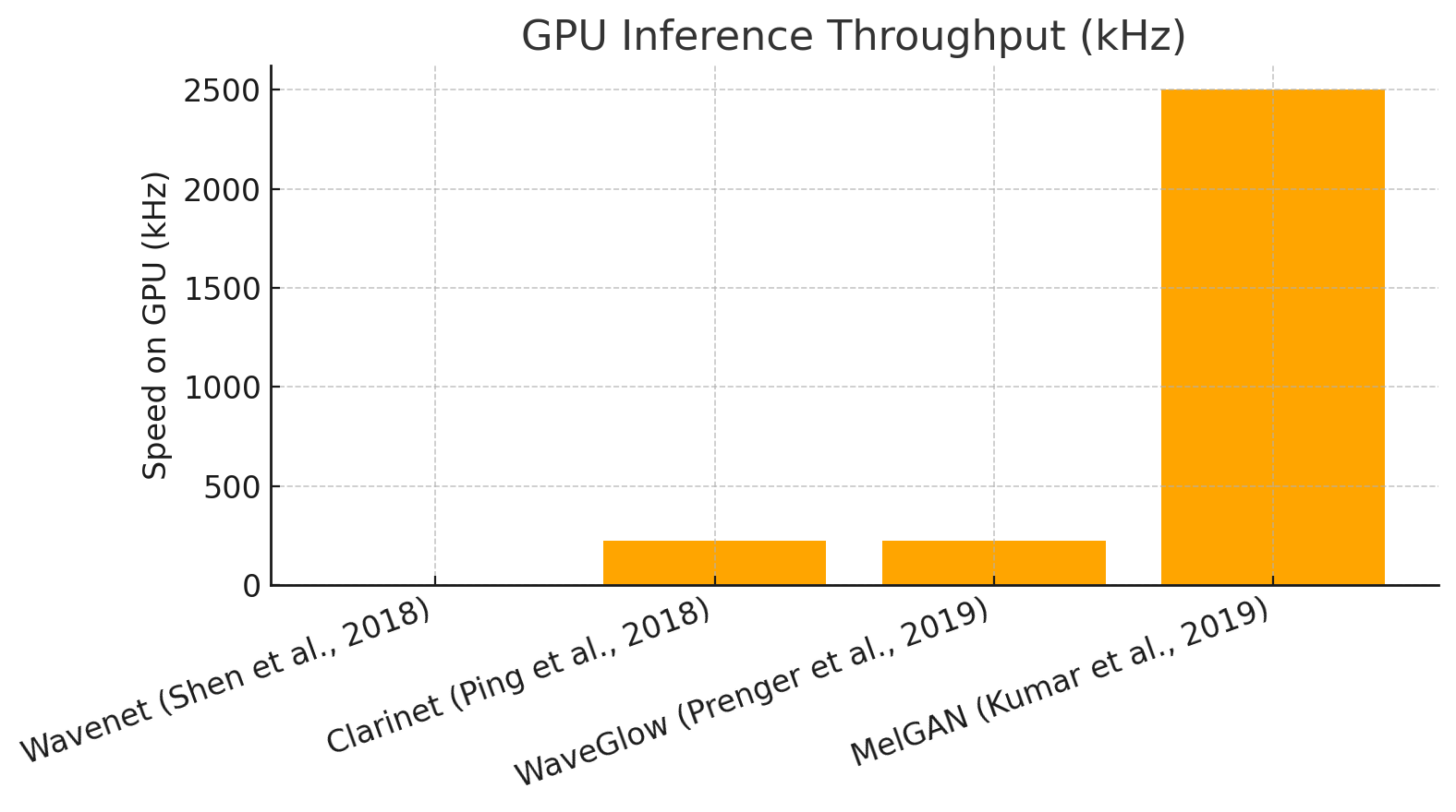
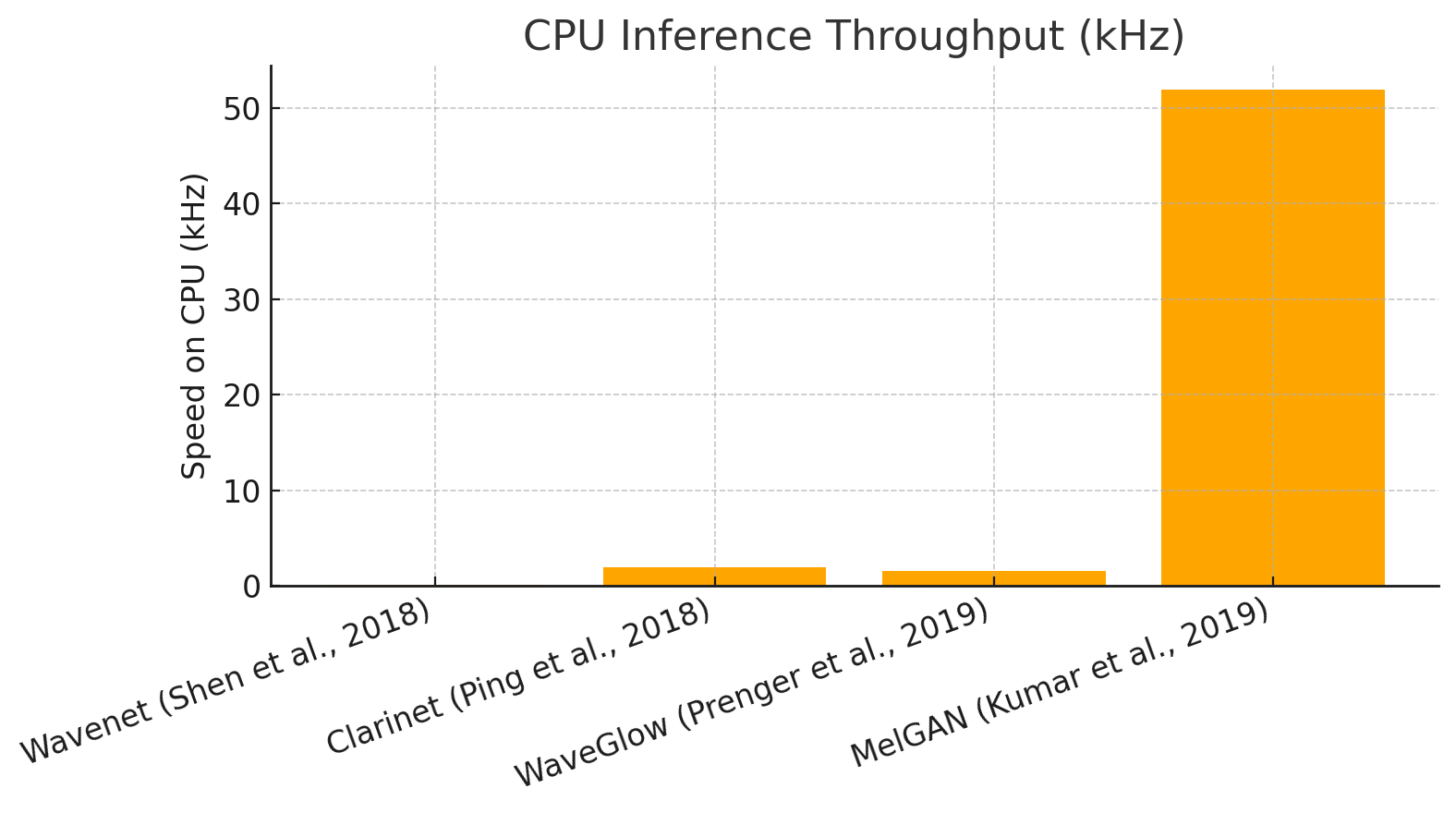
So, why GAN? As we’ve established before, audio data is quite hard to predict. Previous approaches involved autoregression (WaveNet, WaveRNN), or making the model big and complicated (WaveGlow, which took a week of training on 8 GPUs to converge a single speaker, and inference is slow).
There’s a third one, however: adversarial training. Because during training the discriminator keeps helping the generator improve and vice-versa, you can get away with a relatively lightweight model for the G, which is going to be used during inference, and focus most of the complexity on the D, which is discarded after training.
Once MelGAN (and ParallelWaveGAN) showed up and let everyone know that GAN vocoders are indeed possible, they quickly started improving. I got into machine learning circa 2020, so here’s a super compressed timeline based on what was important to me:
Multi-Band MelGAN (Yang et al., 2020): Increased the receptive field of the generator, replaced feature matching loss (commonly used in GANs for stability) with multi-resolution STFT loss, added generator pretraining, and most importantly increased efficiency by generating several sub-bands of audio in parallel (via PQMF filter banks) and then recombining them into a signal, greatly improving speed.
HiFi-GAN (Kong et al., 2020): The real leap. Introduced multi-period discriminators (catching periodicity like pitch/harmonics) alongside multi-scale discriminators, plus heavy use of feature matching.
iSTFTNet (Kaneko et al., 2022): Built as a modification to HiFi-GAN, its authors observed that directly predicting waveform samples is overkill. Instead, iSTFTNet generates a complex STFT and applies the inverse STFT to reconstruct audio. Because it’s much easier for the model to learn STFT than raw audio, it achieves faster training, inference and better quality at smaller sizes.
Quick note: In 2021 a paper stated Multi Resolution Discriminator is all you need, where they took out the Multi-Period Discriminator from HiFi-GAN and found no significant quality degradation.
Said paper is half lie and half truth:
If you’re only doing single speaker, yes, multi resolution discriminator is all you need.
But if you’re doing multi speaker and especially if you want adaptation to unseen speakers, taking out the MPD results in a significant hit to quality, as I observed back then.
The paper comes to the wrong conclusion because they only tested LJSpeech and neglected multispeaker. The lesson here? Run more experiments before claiming something, dummy.
Also, in 2021 I combined the MB-MelGAN generator with the HiFi-GAN discriminator ensemble and found out it performed well.
Of course there’s more, but that’s the important ones, if I listed everything we’d be here forever. And yes, diffusion-based approaches did pop up, but we don’t talk about diffusion here.
Eventually, even the paradigm of what we use for intermediate representation of audio started to change. Remember the humble mel spectrogram?
Mel Spectrograms Out, Latent Spaces In
As I’ve said before, problems the mel spectrogram faced were the immense compression and the loss of phase information, which was especially detrimental to music prediction, but still a big deal in speech.
In response to this the aforementioned models were being adapted into VAEs (Variational auto-encoders, compressing into a smooth, continuous latent space) and VQVAEs (vector quantized, to make into discrete tokens).
VITS (Kim et al., 2021) is a prime example on the VAE side. It fused a variational autoencoder with adversarial training and normalizing flows, letting the model learn a latent space that directly captured speech structure. By gluing together a text-to-speech framework and vocoder (almost a carbon copy of HiFi-GAN), it achieved unparalleled (at the time) audio quality because it skipped the lossy mel spectrogram step.
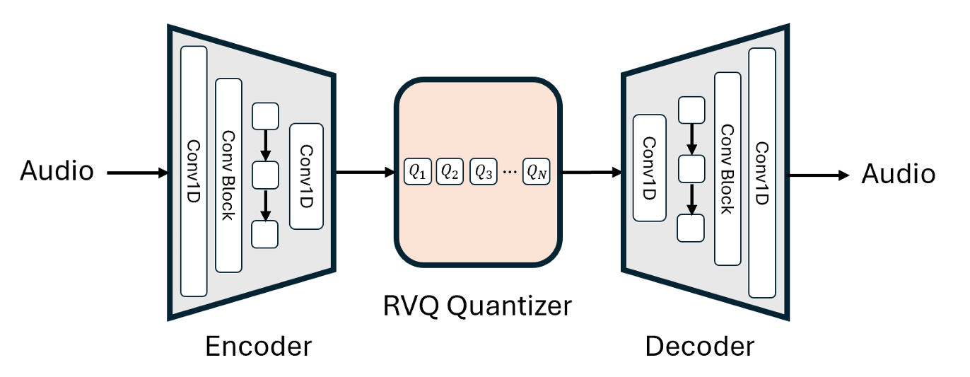
On the VQ-VAE side, two names stand out: SoundStream (Zeghidour et al., 2021) and Descript Audio Codec (Kumar et al., 2023). Both used residual vector quantization to discretize audio into tokens. SoundStream showed you could train an efficient, high-fidelity neural audio codec for speech and music, while Descript Audio Codec, improving from Encodec, greatly improved audio quality and compression with, among other things, the Snake activation function.
We will be dealing exclusively with VQVAEs, because diffusion likes continuous spaces while autoregression (with a sequence model like Transformer or RNN) really prefers discrete ones.
(Yes, I know that discrete diffusion exists, but it’s still experimental at the time I’m writing this)
So, a discerning reader might ask: if the VQ-VAE paper came out in 2017, how did it take so long for discrete audio codecs to pop up?
The original VQ-VAE paper only had a single codebook, and audio data isn’t exactly easy to compress, meaning you had to make said codebook huge (which was impractical because of collapse risk and instability), or accept the crippling bottleneck.
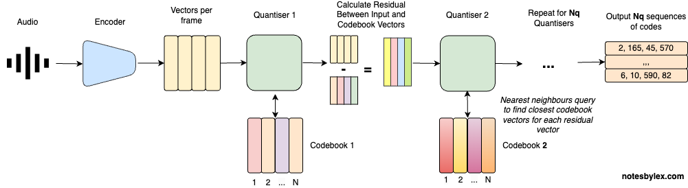
Residual VQ, introduced in the SoundStream paper, solved this by breaking the problem into stages. Instead of one giant codebook, you stack several smaller ones: the first codebook captures the coarse structure, the next captures the residual error, and so on. Now you have a stable way of scaling the bitrate.
It should be noted that all the aforementioned models are GANs, and they use variations of the setup of GAN vocoders before it.
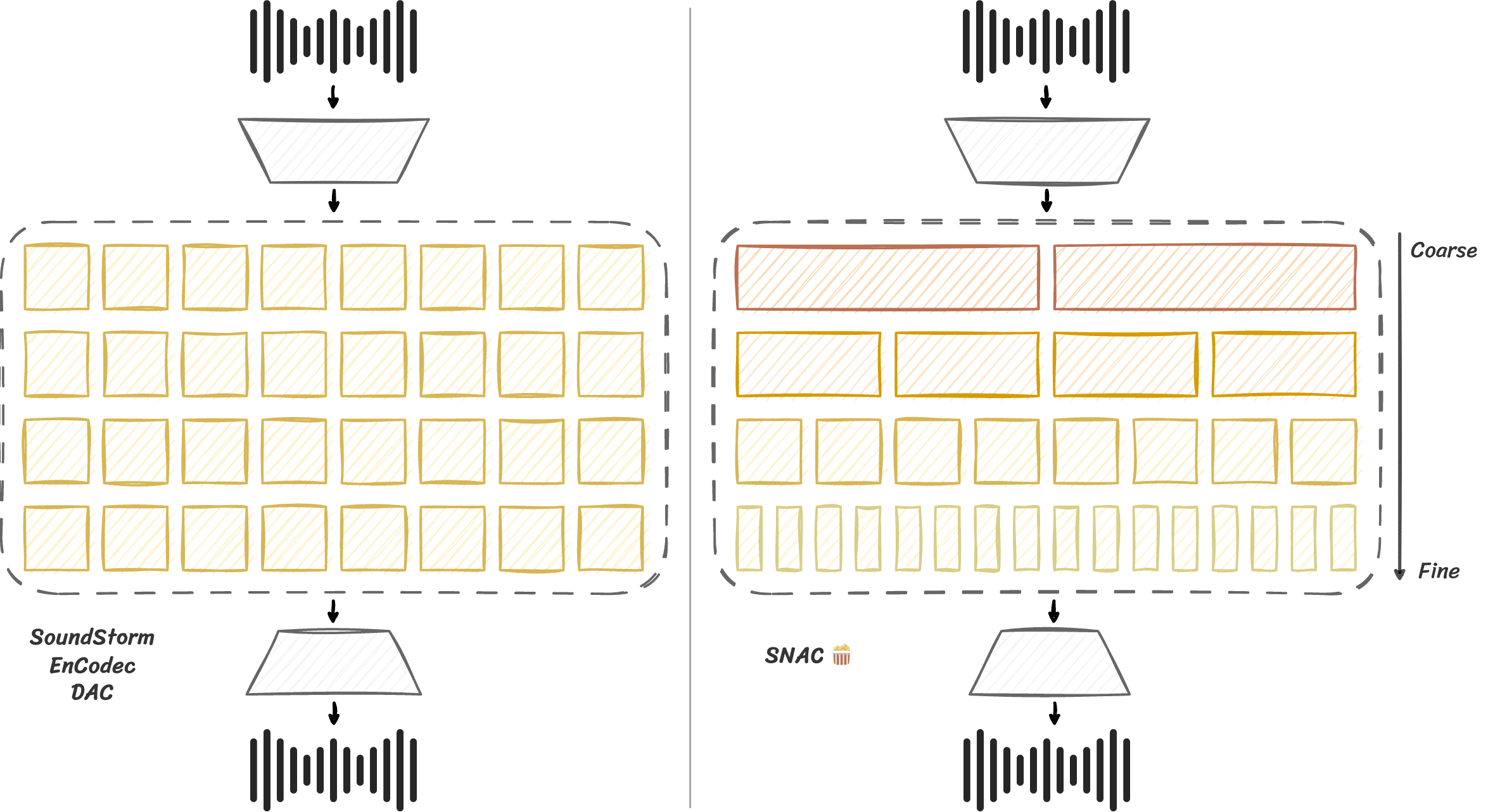
Neural audio codecs like DAC and SNAC (which proposes having coarse/fine tokens) enabled large scale language modeling of audio with Transformers for text-to-speech, spawning models like Zyphra Zonos and Viitor Voice
The Sequence Length Problem
Descript Audio Codec, at 44.1KHz, requires predicting 86 frames per second across 9 codebooks: that is, to predict just one second of audio, the model must predict 774 tokens! With an 8192 context length you can only model 10 seconds of audio.
For reference, in text with a typical LLM tokenizer, that’s the equivalent of 55 paragraphs, 4828 words, 32650 bytes of Lorem Ipsum. You can fit a short book chapter in 8k tokens!
With vanilla attention, sequence length becomes prohibitive after a certain point, due to the quadratic memory complexity — O(N^2). Flash Attention — which virtually everyone who can uses — brings it down to linear, but compute remains quadratic.
Multi-Scale Neural Audio Codec (SNAC), with its multi-scale codes and other tricks that enable much more efficiency, bring speech encoding at 24KHz down to 84 tokens/second. Now you can model 97 (ninety-seven) seconds of audio with 8192 tokens, a dramatic difference.
A bit ago I tried to propose to quantize mel spectrograms first, but ran into issues. The quality loss of mel spectrograms is simply too much to cope
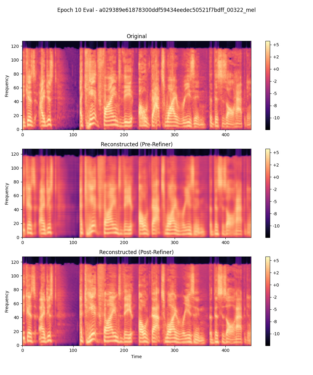
I have another solution cooking, but this has gone on for long enough. Stay tuned for part 2.