
Grouchy: My attempt at trying to use a two-stage approach for audio language modeling
Encode smarter, not harder

(named after Emmanuel de Grouchy, one of Napoleon’s marshals)
Abstract
We introduce Grouchy, a two-stage neural framework for high quality audio language modeling. The first stage employs a lightweight VQGAN that compresses 16KHz audio with FSQ into a compact 132-tokens-per-second discrete representation. The second stage, an adversarially trained Wave U-Net, refines the coarse reconstruction by learning to simultaneously correct and up sample the lossy initial compression into full-band 44.1KHz audio. This separation of coarse structure and fine texture enables Grouchy to achieve good perceptual quality while remaining efficient enough for autoregressive or masked-token generation models. We demonstrate that our approach provides fast convergence and harmonic accuracy without requiring heavy diffusion, scaling, or transformer components, as both of our models are fully convolutional. Grouchy’s modular design positions it as both a practical high-quality neural codec and a bridge toward general-purpose audio language models.
…is what I would say if this model was actually good. It sucks lmao
Introduction
Early neural audio codecs emerged from a desire to replace hand-crafted transforms such as mel spectrograms, with learned latent representations. SoundStream (Zeghidour et al., 2021) demonstrated that an end-to-end convolutional encoder-decoder trained with adversarial and perceptual losses could outperform classical codecs like Opus, introducing the now-standard residual vector quantization (RVQ) stack. Shortly thereafter, Encodec (Défossez et al., 2022) generalized this design, improving stability and bitrate scalability. Neural audio codecs enabled not only compression, but also audio language modeling, such as Descript Audio Codec (Kumar et al., 2023), which was used for modeling 44.1KHz audio.
But, while the aforementioned models far surpassed handmade methods, they were still heavy to use. A second of audio with the aforementioned DAC requires predicting 86 frames per second across 9 codebooks: that is; to synthesize just one second of audio, the model must predict 774 tokens. This quickly becomes prohibitive without tricks.
Related Work
To alleviate this, several ways have been developed. SNAC (Siuzdak et al., 2024) greatly increased efficiency by splitting codebooks into different temporal levels. BigCodec (Xin et al., 2024) showed that scaling the model to about 159M parameters and adding an LSTM was enough to accurately compress 24KHz audio at a bitrate of 1.04k. Most recently, NeuCodec (Julian et al., 2025) scaled the model further to 839M parameters, added multiple feature extractors and a transformer, achieving merely 0.8kbps with a single codebook.
While these have been effective in achieving higher compression, they either rely on scaling (BigCodec), complexity, or both (NeuCodec, SNAC). Additionally, they all compromised on sampling rate, delivering only 24KHz for speech.
A Two-Stage Convolutional Codec
Our theorem is simple: while all the methods above have tried to be a one-in-all, that is, decode the entire and final waveform from the tokens alone, we theorize, given the previous success of audio super resolution models, that we can split the process into two stages:
Base audio stream: A low-bitrate, low-quality stream that encodes rough audio
Refiner: An audio-to-audio model that repairs and restores full-band detail from the base audio inputs
STFT VQGAN
Our first stage consists of a 1D ResNet-based VQGAN that compresses small-hop STFT.
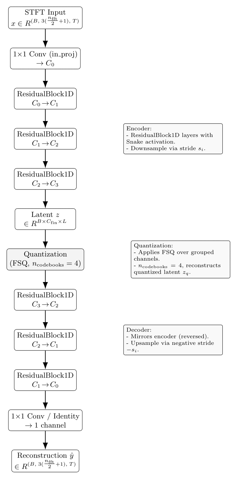
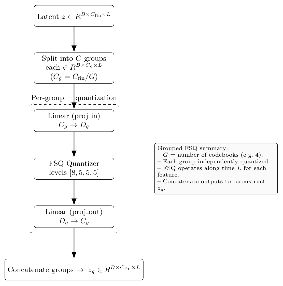
For the quantization scheme, we use grouped finite-scalar quantization, which splits the last hidden states into N groups of equal sizes, vector quantizes each independently, and then concatenates back together channel-wise
Specifically, we extract the STFT of the audio, and express it in three channels: log-mag, sin and cos of phase. Since we are using 1D convolutions, we then flatten the frequency channels.
Therefore, our input and output shape is defined as:
We represent phase as separate sine and cosine components, since these are easier for the model to regress than raw phase angles1; the full phase is later reconstructed using atan2.
After that, the inverse STFT operation is used to recover the waveform.
As per best practices, we use Snake activations everywhere, weight normalization, and a 1D CBAM at the end of every residual block.
(not shown here: we add an eps term to stabilize the log)
The Importance of STFT Params
We use an n_fft, window_size of 16, and a hop_size of 8, representing just 9 frequency bins (27 channels after flattening). This is because we are using 1D convolutions, and a small STFT keeps most of the complexity on the time dimension, allowing us not to need to use Conv2d, which would make it more computationally expensive.
Specifically, we were inspired to do this approach by iSTFTNet (Kaneko et al., 2022), which noted that a large frequency dimension actually reduced performance, even with equivalent compute.
Training VQGAN
For our dataset, we use ~600 hours of utterances from scraped podcasts. We use the Adam optimizer with a learning rate of 0.0001, no weight decay, and 7500 steps of linear LR warmup. We downsample all audio to 16KHz.
For adversarial training, we follow almost the exact same recipe as HiFi-GAN: multi-period and multi scale discriminators2 , and hinge GAN loss.
As for the key difference, we observed that the generator would quickly overpower the discriminator during training and the audio would improve very slowly if at all. Therefore, we follow the Two Time-Scale Update Rule and set the discriminator’s learning rate to 4x that of the generator’s. With this change, the D quickly adapts and keeps challenging the G, resulting in healthy GAN training.
Our perceptual loss cocktail is as follows. We use Multi-Scale Mel loss from Descript Audio Codec, MR-STFT loss from Multi-Band MelGAN, and losses on the direct predicted STFT. Notably we avoid losses directly on the waveform domain.
Another difference from HiFi-GAN is that we down-weight feature matching loss to 0.1 and rely on MR-STFT instead, as the Multi-Band MelGAN paper proposes getting rid of feature matching entirely. This is because feature matching is mainly a training stabilizer, and heavy use of it: forcing the generator to match mean statistics in the D’s feature space, might hurt fine detail especially if the dataset is diverse. We also use Charbonnier loss instead of L1.
Our pitch loss term uses PESTO. We were inspired to do this by a 2020 issue comment on the kan-bayashi/ParallelWaveGAN repo, where someone observed improving quality by using torchcrepe loss. We do MSE between the predicted F0 values of ground truth and predicted, and observe better quality and pitch accuracy.
The batch size is 16. We use a single AMD Instinct MI300X, thanks to Hot Aisle. We train a model to downsample a small STFT of 16KHz audio about 64x by feeding randomly sampled audio chunks of size 16384 samples (a bit more than a second at 16KHz), with the final latent being split into 4 codebooks. The generator has ~30M parameters and is fully convolutional. Therefore, with 33 fps and 4 codebooks size 1000, the bitrate is 132 tok/s, or 1.32 kbps.
We pretrain the generator for 130k steps. The training process to 1.2M total steps took about 3 days. Here is an evaluation sample:
Ground truth:
Reconstructed:
As you can see, the voice identity is preserved, but the audio quality itself is greatly degraded. This is where our second stage comes in.
Wave U-Net Corrector
Since we’ve already observed good results previously with U-Nets (see MQGAN Refiner), we decide to go with a Wave U-Net, which is proven to work for a variety of audio-to-audio tasks, including stem separation, speech dereverberation/denoising, et al.
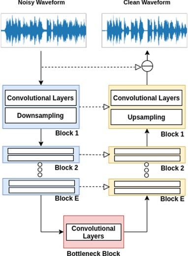
We did experiment with U-Net in the STFT domain but found the performance to be unsatisfactory as opposed to raw audio. Once again, we are using weight normalization and Snake activations in the G. Following best practices in Wave U-Nets, we use a kernel size of 15 in the encoder, and 5 in the decoder, using linear upsample + conv instead of deconvolution.
Since the U-Net’s task is to correct audio degraded by the compression process and restore full-band detail, our data preparation consisted of passing all of our audio through the pretrained VQGAN, naively upsampling to 44.1KHz, and saving the processed version. The model’s dataloader is then made to give pairs of degraded and ground truth audios. We use a chunk size of 16384 again and observe that going higher resulted in more training time but no increase in quality.
Our training process is identical to the VQGAN’s, just with some perceptual loss parameters updated to reflect 44.1KHz audio.
We pretrain the generator for 60k steps, and after a total of 280k steps, or 15 hours, the training is done.
Here is it after being fed the coarse reconstruction previously:
Limitations & Conclusion
The training dataset was very small, and a lot of it is audio of dubious quality, and the base model kind of sucks regardless. I don’t have the resources to roll my own audio neural audio codec anyway, so I’ll use someone else’s. This was just my foray into it.
I would like to thank Hot Aisle for the GPU compute. I’m doing all of this in PyTorch ROCm, and the only problem I ran into was some kernel turning stubborn and erroring out (with torch.backends.cudnn.benchmark = True) after I made a few too many changes to a model, so I fixed it by doing rm -rf $HOME/.cache/miopen. Otherwise, I hope to have proven you can do real machine learning work on AMD GPUs.
Source: Google Gemini said so
We are aware that newer discriminators have been proposed, but we didn’t have proper time to ablate. Therefore, following our constraints, we went with the tried-and-true recipe.