


Activation Functions, Part 2
Now with simple benchmarks and stuff.

Recap
This expands on my previous post, where I proposed two activation functions:
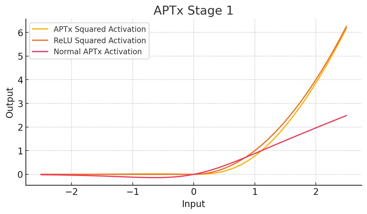
APTx Stage 1
ReLU GT (Gradient Touring)
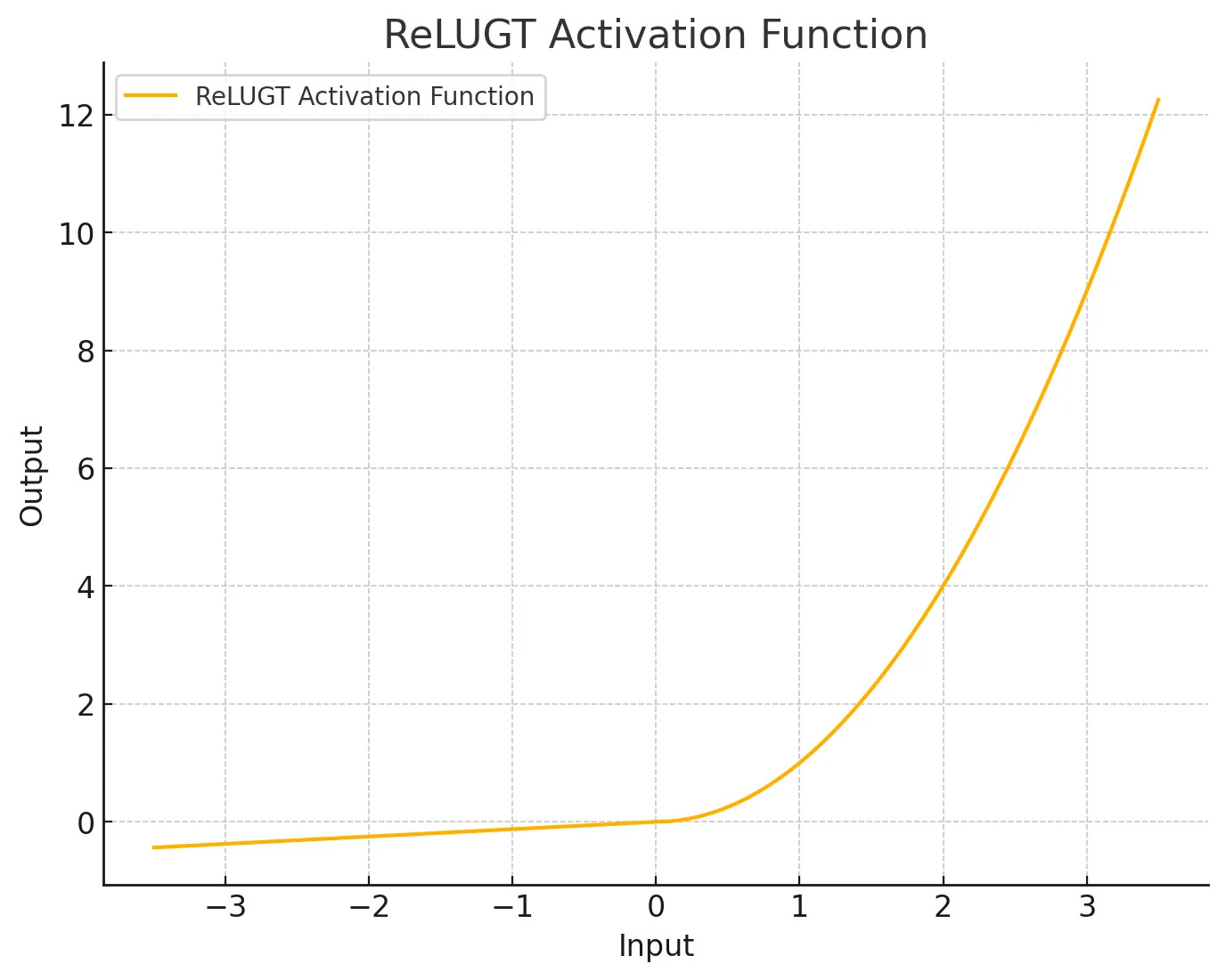
This time I’ll be most focused on ReLUGT. To recall:
It has a trainable negative slope (initialized to 0.05), a static negative alpha (2.5), and a trainable positive alpha (1.0), squaring the positive part. I have no mathematical justification for this function, I just built it based on what I noticed that the gradient likes.
Now, I am here to provide at least small-scale results that I did with free T4s in Google Colab.
The Setup
I took the IMDB classification dataset, and made a small, simple model:
1x Embedding (input is characters) → 4-Layer Transformer Encoder → Avg Pooling → Linear
The model is trained with BCEWithLogitsLoss objective. The Transformer has 4 heads and everything 256 dim, the batch size is 64, and the dataset is split with sklearn’s train_test_split with a fixed random_state number to ensure every run has the same split.
I train up to 10 epochs three times per activation function, then note down the validation accuracy for each run and take the average of those three runs to account for the stochasticity of model training.
But before I show the results, let me sell you some car insurance on my theory
The Argument for Parametric Activation Functions
Parametric activation functions are activation functions that include trainable parameters which allow autograd to adjust it on the fly. To quote my previous post:
Notably, the KAN vs MLP paper noted that a big advantage of KANs is specifically their parametric activation function, and that when they did the same with MLPs, their performance also improved.
Right now, there is no exploration of parametric activation functions in Transformers — except for the GLU variants, which involve gating, that kind of counts.
My instinct says: there is big unexplored potential in them, especially because Transformer architectures learn to specialize layer-by-layer on different features, and this has been studied, at least for BERT1


I don’t know if it has been studied for LLMs, but you can go here for an interactive LLM visualization and try to spot it.
Once again, my instinct says: due to the aforementioned realities, parametric activation functions in the feed-forward would afford the gradient flexibility to optimize much more efficiently per-layer. Interestingly enough, this started out with me just trying to figure out something better than ReLU squared.
Now, it is time to get to some small-scale results.
Results
I noted down all the val accs into Excel because I had a period between 2018 - 2020 where I was obsessed with statistics and so I became comfortable with it.

Y is validation accuracy, X is epoch number.
ReLU2 is ReLU squared, the conventional go-to activation function when the GLU variants add too many parameters
APTXS1-T is APTx Stage 1 with trainable beta and alpha parameters
ReLUGTz is ReLUGT, but with the 2x expansion and gating of a GLU variant.
ReLUGT and SwiGLUFFN don’t require explanation
For some reason, SwiGLU underperforms on this test. I suspect this is because such a small-scale task doesn’t really benefit from the additional parameters and complexity it provides, but ReLUGTz integrates the same complexity and scores the best (???)
All activations converge similarly, but the most glaring difference is the speed: ReLUGTz is the fastest in this regard, followed closely by its lighter cousin ReLUGT; ReLU squared is dead last.
For another perspective, I also did a sum of the accuracies.

Now, despite this, SwiGLU does perform best on the test case (after ten epochs), which I will attribute to faster convergence enabling earlier overfitting. 10 whole epochs is kind of overkill for this task, or bad luck. That’s actually because the testing is done with the best eval loss model, which SwiGLU’s is more trained because it’s smoother. (I’ll rerun this later)
Deeper
Since it shows promise, I’m going to focus on ReLUGT, which was originally just a byproduct of me adapting the APTx function to be trainable then squared.

This is a plot of what each FFN layer’s activations look like after training up to 10 epochs — these are learned activations. (there’s another graph but more pronounced in my previous post)
Now, there’s not that much variation because this is a very simple task and model (this Transformer doesn’t even have positional encodings!), but we can see a certain pattern begin to emerge. Meaning, the model does learn a smooth distribution of curves.
Moreover, the differences on the negative part are more pronounced than the positive, which could explain the performance gap between ReLUGT and APTx S1 — the former lets negative values in and provides a smooth optimization path, while the latter doesn’t.
Conclusion
Here I’ve proposed and did some preliminary testing of some activation functions, along with theory, and they look promising to me.
But do take this with a grain of salt. This is on a toy task; I don’t know how well it’ll scale up — I have some idea since APTx S1 annihilated ReLU Squared in my TTS model — but not much beyond that.
Next step is to try pretraining a smaller BERT or GPT-2 and comparing. If it does scale up well, and this is a big if — it could change the paradigm.
Fuck, I need compute.
Transparency
Now, unlike that Reflection 70B shithead, I ain’t no grifter: Here are Colab notebooks so you can reproduce it. Don’t email the account that owns these notebooks, you won’t get a reply.
Here is the code for each function too:
class ReLUGT(nn.Module):
    """
    ReLU GT: Leaky squared ReLU with trainable positive alpha, slope, and static negative alpha.
    """
    def __init__(self, initial_slope=0.05, initial_alpha_neg=2.5, initial_alpha_pos=1.0):
        super(ReLUGT, self).__init__()
        self.slope = nn.Parameter(torch.tensor(initial_slope))
        self.alpha_neg = initial_alpha_neg
        self.alpha_pos = nn.Parameter(torch.tensor(initial_alpha_pos))

    def forward(self, x):
        return torch.where(x < 0, self.alpha_neg * self.slope * x, self.alpha_pos * x ** 2)


class ReLUGTzFFN(nn.Module):
    def __init__(self, embed_dim, hidden_dim, dropout=0.1):
        super(ReLUGTzFFN, self).__init__()
        # The gated linear unit
        self.linear1 = nn.Linear(embed_dim, hidden_dim * 2)  # doubled hidden_dim for gating
        self.dropout = nn.Dropout(dropout)
        self.linear2 = nn.Linear(hidden_dim, embed_dim)
        self.dropout2 = nn.Dropout(dropout)
        self.relugt = ReLUGT()

    def forward(self, x):
        # Linear transformation followed by gating mechanism
        x = self.linear1(x)
        hidden_dim = x.size(-1) // 2
        x1, x2 = x[..., :hidden_dim], x[..., hidden_dim:]  # Split into two halves
        x = self.relugt(x1) * x2  # ReLUGT and gating
        x = self.dropout(x)
        x = self.linear2(x)
        x = self.dropout2(x)
        return x


class APTxS1(nn.Module):
    """
    APTx Stage 1:

    - Trainable beta and gamma (allows model to dynamically adjust upwards slope and scaling)
    - Squaring output, inspired by Squared ReLU.
    """

    def __init__(self, alpha=1.0, beta=1.0, gamma=0.5, trainable=True):
        super(APTxS1, self).__init__()
        self.alpha = alpha
        if trainable:
            self.beta = nn.Parameter(torch.tensor(beta, dtype=torch.float32))
            self.gamma = nn.Parameter(torch.tensor(gamma, dtype=torch.float32))
        else:
            self.beta = beta
            self.gamma = gamma

    def forward(self, x):
        return ((self.alpha + torch.tanh(self.beta * x)) * self.gamma * x) ** 2